Billion Messages - Art of Architecting scalable ElastiCache Redis tier

Whenever we are designing a highly scalable architectures on AWS running thousands of application servers and supporting millions of requests, usage of NoSQL solutions have become inevitable part. One such solution we often been using for years on AWS is Redis . We love Redis. 
AWS introduced ElastiCache Redis on 2013 and we started using the same since it eased the management and operational efforts.  In this article i am going to share my experience on designing large scale Redis tiers supporting billions of messages per day on AWS, step by step guide on how to deploy the same, what are the Implications you face at scale ? Best Practices to be adopted while designing sharded+replicated Redis Tiers etc.

Since we need to support billions of message requests per day and it was growing:

• the ElastiCache Redis tier was designed with Partitions( shards) to scale out as the customer grows
• the ElastiCache Redis tier was designed with Replica Slaves for HA and read scaling as the read volumes grow

When your application is growing at Rapid pace and lots of data are created every day, you cannot keep increasing (scaling up) the size of the ElastiCache Node. At one point you will hit the maximum memory capacity of your EC2 instance and you will be forced to partition.  Partitioning is the process of splitting your Key Value data into multiple ElastiCache Redis instances, so that every instance will only contain a subset of your Key Value pair. It allows for much larger ElastiCache Redis data stores, using the sum of the memory of many ElastiCache Redis Nodes. It also allows to scale the computational power to multiple cores and multiple EC2, and the network bandwidth to multiple EC2 network adapters. There are two widely used partition/shard implementation techniques that are available for ElastiCache Redis Tier :
Technique 1) Client side partitioning means that the Redis clients directly select the right ElastiCache Redis node where to write or read a given key. Many Redis clients implement client side partitioning, chose the right one wisely.
Technique 2) Proxy assisted partitioning means that your clients send requests to a proxy that is able to speak the Redis protocol, which in turn sends requests directly to the right ElastiCache Redis instance. The proxy will make sure to forward our request to the right Redis instance accordingly to the configured partitioning schema. Currently the most widely used Proxy assisted partitioning tool is Twemproxy , written by Manju Raj of twitter. Git hub link https://github.com/twitter/twemproxy . Twemproxy is a proxy developed at Twitter for the Memcached ASCII and the Redis protocol. Twemproxy supports automatic partitioning among multiple Redis instances and  currently it is the suggested way to handle partitioning with Redis.

In this article we are going to explore in detail about Proxy assisted partitioning technique for highly scalable and available Redis tier.

Welcome to Twemproxy
Twemproxy( nutcracker) is a fast single-threaded proxy supporting the Memcached ASCII protocol and more recently the Redis protocol.

Installing Twemproxy:
Download the Twemproxy package.
wget http://twemproxy.googlecode.com/files/nutcracker-0.3.0.tar.gz
tar -xf nutcracker-0.3.0.tar.gz
cd nutcracker-0.3.0
./configure
make
make install

Configuration:
Twemproxy (Nutcracker) can be configured through a YAML file specified by the -c or --conf-file command-line argument on process start. The configuration file is used to specify the server pools and the servers within each pool that nutcracker manages. The configuration files parses and understands the following keys:

• listen: The listening address and port (name:port or ip:port) for this server pool.
• hash: The name of the hash function.
• hash_tag: A two character string that specifies the part of the key used for hashing. Eg "{}" or "$$". Hash tag enable mapping different keys to the same server as long as the part of the key within the tag is the same.
• distribution: The key distribution mode.
• timeout: The timeout value in msec that we wait for to establish a connection to the server or receive a response from a server. By default, we wait indefinitely.
• backlog: The TCP backlog argument. Defaults to 512.
• preconnect: A boolean value that controls if nutcracker should preconnect to all the servers in this pool on process start. Defaults to false.
• redis: A boolean value that controls if a server pool speaks redis or memcached protocol. Defaults to false.
• server_connections: The maximum number of connections that can be opened to each server. By default, we open at most 1 server connection.
• auto_eject_hosts: A boolean value that controls if server should be ejected temporarily when it fails consecutively server_failure_limit times. See liveness recommendations for information. Defaults to false.
• server_retry_timeout: The timeout value in msec to wait for before retrying on a temporarily ejected server, when auto_eject_host is set to true. Defaults to 30000 msec.
• server_failure_limit: The number of consecutive failures on a server that would lead to it being temporarily ejected when auto_eject_host is set to true. Defaults to 2.
• servers: A list of server address, port and weight (name:port:weight or ip:port:weight) for this server pool.

For More details Refer: https://github.com/twitter/twemproxy

Running and Accessing Twemproxy 
To start the proxy just use the command “nutcracker” with the configuration file path specified or in its default path(conf/nutcracker.yml) .
Based on the configuration the twemproxy will be running and listening. Configure your application to point to the port and address instead of the Redis cluster.

Twemproxy Deployment models:

We usually deploy Twemproxy one one of the following models in AWS :
Model 1: Twemproxy as a separate Proxy Tier: In this model Twemproxies are deployed in separate EC2 instances, The application tier is configured to point to Twemproxies . The Twemproxy tier in turn maintains the mappings to the ElastiCache redis nodes. It is better to use instances with very good IO bandwidth for twemproxy tier in AWS. In case you feel the instance CPU is underutilized, you can launch multiple Twemproxy instances inside the same single EC2 instance as well.

Though the above model looks clean and efficient there are optimizations that can be applied to this architecture :
What happens when the twemproxy01 fails, how will the Application server instances know about it ?
Why should i pay additional for twemproxy EC2 instances, Can it be minimized ?

Model 2 : Twemproxy bundled with application tier EC2's: In this model twemproxies are bundled in the same box of the application server EC2 itself. Since two twemproxies are not aware of each others existence, it is easy to architect this model even in App->Auto Scaling mode. Every application server talks to the local twemproxy deployed in the same box this saves cost and avoids managing additional tier complexity as well.

Reference ElastiCache Redis + Twemproxy  deployment:
(This is a Reference deployment, the same can be scaled out to hundreds depending upon the need. It is a Redis Partitioned + replicated setup )
1. Two ElastiCache Redis nodes in AWS (twem01 and twem02)
2. Replication group for each ElastiCache redis nodes (twem01-rg and twem02-rg with one Read Replica each)
3. Two twemproxy servers running in separate EC2. (twemproxy01 and twemproxy02)
Once the above setup is done please note down the endpoints. We will be using the Replication group endpoint as the ElastiCache Redis endpoint for the twemproxy.

ElastiCache Redis Endpoints:
twem01-twem01.qcdze2.0001.usw2.cache.amazonaws.com:6379
twem02-twem02.qcdze2.0001.usw2.cache.amazonaws.com:6379
ElastiCache Redis Replication endpoints:
twem01-rg.qcdze2.ng.0001.usw2.cache.amazonaws.com:6379
twem02-rg.qcdze2.ng.0001.usw2.cache.amazonaws.com:6379

To test the Twemproxy we pumped following keys:
Pump KV data through the Twemproxy01 (1-2000 keys)
Pump KV data through the Twemproxy02(2001-4000 keys).

Configuration:
beta:
  listen: 127.0.0.1:22122
  hash: fnv1a_64
  hash_tag: "{}"
  distribution: ketama   #Consistent Hashing
  auto_eject_hosts: false
  timeout: 5000
  redis: true
  servers:
- twem01-rg.qcdze2.ng.0001.usw2.cache.amazonaws.com:6379:1 server1
- twem02-rg.qcdze2.ng.0001.usw2.cache.amazonaws.com:6379:1 server2

Test 1: Testing Key accessibility . Testing "GET" operation across both the Twemproxy Instances for few sample keys. 

Fetch 4 Keys spread across 4000 KV data from Twemproxy01  EC2 instance:
[root@twemproxy01 redish]# src/redis-cli -h 127.0.0.1 -p 22122
redis 127.0.0.1:22122> get 1000
"1000-data"
redis 127.0.0.1:22122> get 2000
"2000-data"
redis 127.0.0.1:22122> get 3000
"3000-data"
redis 127.0.0.1:22122> get 4000
"4000-data"
Fetch 4 Keys spread across 4000 KV data from Twemproxy02  EC2 instance:
[root@twemproxy02 redish]# src/redis-cli -h 127.0.0.1 -p 22122
redis 127.0.0.1:22122> get 1000
"1000-data"
redis 127.0.0.1:22122> get 2000
"2000-data"
redis 127.0.0.1:22122> get 3000
"3000-data"
redis 127.0.0.1:22122> get 4000
"4000-data"

From the above test it is evident that all 4000 KV data inserted using both Twemproxies are accessible from both Twemproxies( testing the sample) even though they are not aware among themselves. This is because of the same hashing and Key mapping translation done at Twemproxy level.

Test 2: Testing the ElastiCache Redis Availability and Fail over mechanism:

We are going to promote the twem01-rg replication group read replica to be the Primary Redis Node. After promotion we are going to test:

1. Whether the Twemproxy is able to recognize the newly promoted master
2. Whether the sample KV data is safely replicated and still accessible , to ensure failover is successful.

To promote ElastiCache Redis slave just click the promote Action and confirm or automate using API. During the promotion of Read Replica to master we observed that the transition happens very quickly and there is no timeout but the response time for the query is about 4-5 secs for about 3-4 minutes during the switch over. In the Twemproxy configuration we can set the timeout configuration, this value needs to be set accordingly so that during switch over there will be no connection refused. For the sample test we have set it as 5000

Repeat Test 1:

[root@twemproxy01 redish]# src/redis-cli -h 127.0.0.1 -p 22122
redis 127.0.0.1:22122> get 1000
"1000-data"
redis 127.0.0.1:22122> get 2000
"2000-data"
redis 127.0.0.1:22122> get 3000
"3000-data"
redis 127.0.0.1:22122> get 4000
"4000-data"
Fetch 4 Keys spread across 4000 KV data from Twemproxy02  EC2 instance:
[root@twemproxy02 redish]# src/redis-cli -h 127.0.0.1 -p 22122
redis 127.0.0.1:22122> get 1000
"1000-data"
redis 127.0.0.1:22122> get 2000
"2000-data"
redis 127.0.0.1:22122> get 3000
"3000-data"
redis 127.0.0.1:22122> get 4000
"4000-data"

From the above test it is evident that all 4000 KV data are replicated properly between master and slaves nodes and the transition between slave to master happened successfully with all the data.

Reporting

Nutcracker exposes stats at the granularity of server pool and servers per pool through the stats monitoring port. The stats are essentially JSON formatted key-value pairs, with the keys corresponding to counter names. By default stats are exposed on port 22222 and aggregated every 30 seconds.

Some best practices while designing highly scalable+available ElastiCache Redis Tier :

Practice 1 : Reduce the Number of Connections and pipeline messages:
Whenever the application instance gets a request to get/put value to the ElastiCache redis node, the client makes a connection to the Redis Tier. Imagine it is a heavy traffic site, then thousands of requests hitting translates to thousands of connections from the application instance to Redis Tier. Now when you add Auto- scaling to your application tier and you have few hundred servers scaled out , then imagine the connection complexity and overhead this architecture brings to the ElastiCache Redis Tier.

Best practice is minimize the number of connections made from your application instance to your ElastiCache redis node. Use Twemproxy in bundled mode with Application EC2 instance, this keeps the process in close proximity and reduces the connection overhead.  Secondly, Twemproxy internally uses minimal connections to ElastiCache Redis Instance by proxying multiple client connections onto one or few server connections.
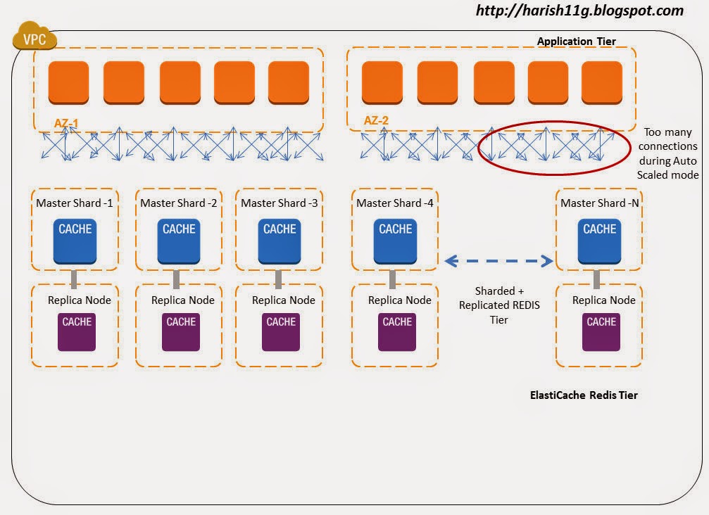
Redis also supports pipelines, where multiple requests can be pipelined and sent on a single connection. In a simple test using large Application & ElastiCache node we were able to process 125K message/sec in pipeline mode, now imagine what you could achieve on bigger instance types on AWS. The connection minimization architectural setup of twemproxy makes it ideal for pipelining requests and responses and hence saving on the round trip time.  For example, if twemproxy is proxying three client connections onto a single server and we get requests - 'get key\r\n', 'set key 0 0 3\r\nval\r\n' and 'delete key\r\n' on these three connections respectively, twemproxy would try to batch these requests and send them as a single message onto the server connection.

Note : It is important to note that "read my last write" constraint doesn't necessarily hold true when twemproxy is configured with server_connections: > 1. Let us consider a scenario where twemproxy is configured with server_connections: 2. If a client makes pipelined requests with the first request in pipeline being set foo 0 0 3\r\nbar\r\n (write) and the second request being get foo\r\n (read), the expectation is that the read of key foo would return the value bar. However, with configuration of two server connections it is possible that write and read request are sent on different server connections which would mean that their completion could race with one another. In summary, if the client expects "read my last write" constraint, you either configure twemproxy to use server_connections:1 or use clients that only make synchronous requests to twemproxy.

Practice 2:  Configure Auto Ejection and Hashing combination properly
Design for failure is the mantra of cloud architecture. Failures are commons when things are distributed on scale. Though partitioning when using ElastiCache Redis as a data store or cache is conceptually the same on broad lines, there is a huge difference operationally on large scale systems. When you are using ElastiCache Redis as a data store you need to be sure that a given key always maps to the same instance, Whereas if you are using  ElastiCache Redis as cache if a given node is not available, then you can always start afresh using a different node in the hash ring with consistent hashing implementations.
To be resilient against failures, it is recommended that you configure Auto eject hosts false when you treat redis as a Data Store and true in when you treat redis as a cache.
resilient_pool:
  auto_eject_hosts: true
  server_retry_timeout: 30000
  server_failure_limit: 3
Enabling auto_eject_hosts: This property ensures that a dead ElastiCache redis Node can be ejected out of the hash ring after server_failure_limit: consecutive failures have been encountered on that node. A non-zero server_retry_timeout: ensures that we don't incorrectly mark a node as dead forever especially when the failures were really transient. The combination of server_retry_timeout: and server_failure_limit: controls the tradeoff between resiliency to permanent and transient failures.
Note that an ejected node will not be included in the hash ring for any requests until the retry timeout passes. This will lead to data partitioning as keys originally on the ejected node will now be written to another node still in the pool. If ElastiCache Redis is used as a cache (in memory) then in event of a Redis Node going down, the cache data will be lost. This cache miss can cascade performance problems to other tiers and altogether bring down your system on the cloud. To minimize KV cache miss,  you can design your hash ring with Ketama hashing on the Redis Proxy. This will minimize the Cache miss in event of cache node failure, also it decreases the overall re-balancing needed in your Redis tier.  In addition to helping hand on availability problems, Redis Proxy+Ketama can also help your Redis farm to Scale out and Scale down easily with minimal cache miss. To know more about Ketama on ElastiCache refer http://harish11g.blogspot.com/2013/01/amazon-elasticache-memcached-internals_8.html  . The below diagram illustrates a ElastiCache Redis Cache Farm with Consistent Hash Ring.

In short to minimize the cache miss when using auto eject with true it is recommended to use "Ketama Hashing ( Consistent Hashing Algorithm)" on your Twemproxy configuration. 

ElastiCache Redis as a Data Store:
What if the data stored in your Cache is important and needs to persisted across node failures and launch ? What if the date stored in your Cache cannot be lost and it needs to be replicated and promoted during failures?
Welcome to ElastiCache Redis as Data store. ElastiCache Redis offers features to persist the in memory cache data to disk and also replicate it to a slave for high availability. If ElastiCache Redis is used as a store (persistent), you need to keep the map between keys and nodes fixed, and a fixed number of nodes. Since the data stored is important when you treat ElastiCache Redis as a data store, in event one Redis node goes down, you should have immediate standby up and running in minutes.  You can architect ElastiCache Redis master with one or more replication Slave launched on different AZ from Master for High Availability in AWS. In event master node failure or master AZ failure, the slave Redis node can be promoted in minutes to act as master. This whole High availability design keeps the number of nodes on the hash ring stable and simple, Otherwise, you will end up building a system to re balance the keys (which is not easy) between nodes whenever there is a addition or removal of nodes during outages. In addition to above the ElastiCache Redis supports Partial Resynchronization with Slaves - If the connection between a master node and a slave node is momentarily broken, the master now accumulates data that is destined for the slave in a backlog buffer. If the connection is restored before the buffer becomes full, a quick partial resync will be done instead of a potentially longer full resync. This really saves network bottleneck during momentary failures.
In large scale systems you will often find some partitions are heavily used than others , in event the usage is read heavy in nature you can add upto 5 Read replicas for the ElastiCache Redis Master partition. Since these replicas are used only for read they do not affect the Hash ring structure. But Twemproxy lacks the support for read scaling with Redis Replica's. So in event when you face this problem, you will have to Scale up the capacity(instance/node type) of the Master and Slave of that partition alone.

If you are using ElastiCache redis as a Data store in the TwemProxy it is recommended to keep "auto_eject_hosts" property false so that in event of redis node failure it is not ejected from the hash ring. The hash ring can be built with both ketama or modula hash algorithms , since in event of Primary node failure, the Slave is going to be promoted and ring structure is going to be always maintained. But if you feel there is immense possibility for the number of primary node partitions to grow, or major failures to occu, it is better to choose ketama hash ring itself from beginning. The below diagram illustrates the architecture.

Practice 3: Configure the Buffer properly:
All memory for incoming requests and outgoing responses is allocated in mbuf in Twemproxy. Mbuf enables zero copy for requests and responses flowing through the proxy. By default an mbuf is 16K bytes in size and this value can be tuned between 512 and 16M bytes using -m or --mbuf-size=N argument. Every connection has at least one mbuf allocated to it. This means that the number of concurrent connections twemproxy can support is dependent on the mbuf size. A small mbuf allows us to handle more connections, while a large mbuf allows us to read and write more data to and from kernel socket buffers. Large Scale web/mobile applications involving millions of hits might have small size request/response and lots of concurrent connections to handle in their backend. So at such scenarios, when Twemproxy is meant to handle a large number of concurrent client connections, you should set chunk size to a small value like 512 bytes to 1K bytes using the -m or --mbuf-size=N argument.

Practice 4: Configure proper Timeouts
It is always a good idea to configure Twemproxy timeout: for every server pool, rather than purely relying on client-side timeouts. Eg:

resilient_pool_with_timeout:
  auto_eject_hosts: true
  server_retry_timeout: 30000
  server_failure_limit: 3
  timeout: 400
Relying only on client-side timeouts has the adverse effect of the original request having timed out on the client to proxy connection, but still pending and outstanding on the proxy to server connection. This further gets exacerbated when client retries the original request.


Benefits of using Twemproxy for Redis Scaling

• Avoids re inventing the wheel. Thanks Manju Raj (twitter).
• reduce the number of connections to your cache server by acting as a proxy
• shard data automatically between multiple cache servers
• support consistent hashing with different strategies and hashing functions
• be configured to disable nodes on failure
• run in multiple instances, allowing client to connect to the first available proxy server
• Pipelining and batching of requests and hence saving of round-trips

Disadvantages of Partitioning Model:

Point 1) Operations involving multiple keys are usually not supported. For instance you can't perform the intersection between two sets if they are stored in keys that are mapped to different Redis instances (actually there are ways to do this, but not directly).Redis transactions involving multiple keys can not be used.
Point 2) The partitioning granularity is the key, so it is not possible to shard a dataset with a single huge key like a very big sorted set. Ideally in such cases you should Scale UP the particular Redis Master-Slave to larger EC2 instance or pro grammatically stitch up the sorted set.
Point 3)When partitioning is used, data handling is more complex, for instance you have to handle multiple RDB / AOF files, and to make a backup of your data you need to aggregate the persistence files/snapshots from multiple EC2 Redis slaves.
Point 4) Architecting a partitioned + replicated ElastiCache Redis tier not complex. What is more complex is ? supporting transparent rebalancing of data with the ability to add and remove nodes at runtime. Systems like client side partitioning and proxies don't support this feature. However a technique called Presharding helps in this regard with limitations. Presharding technique ->Since Redis is lightweight, you can start with a lot of EC2 instances since the beginning itself. For example if you start with 32 or 64 EC2 instances (micro or small Cache Node instance type)  as your node capacity , it will provide enough room to keep scaling up the capacity when your data storage needs increase. It is not a highly recommended technique. But still can be used in production if your growth pattern is very predictable.

Future of highly scalable + available Redis tiers -> Redis Cluster

Redis Cluster is the preferred way to get automatic sharding and high availability. It is currently not production ready. Once Redis Cluster / Client  is available on Amazon ElastiCache, it will be the de facto standard for Redis partitioning. It uses a mix between query routing and client side partitioning.

References:
http://redis.io/documentation
https://github.com/twitter/twemproxy

This article was co-authored with Senthil

Other Amazon ElastiCache Articles :
Caching architectures using Memcached & Amazon ElastiCache
Highly Available ElastiCache Redis replication cluster in AWS VPC
Deep dive into Amazon Elasticache
Distributed Cache On Steroids: Amazon ElastiCache
Launching Amazon ElastiCache in 3 Easy Steps
AWS Performance Tip 3: Use Amazon ElastiCache to improve application performance

Loading Big Index Data into newly launched Amazon CloudSearch engine

Search tier is the most critical section of many online verticals like travel, e-commerce, classifieds etc. If users cannot search products efficiently they will not make their buying decisions properly, which in turn massively affects the revenues of these companies. Most of them are usually powered by Apache Solr, FAST , Autonomy, ElastiSearch etc.  AWS also has a Search Service called CloudSearch which is a fully-managed service in the cloud that makes it easy to set up, manage, and scale a search solution for your website. Amazon CloudSearch relieves you from the worry of hardware provisioning, setup, and maintenance. As your volume of data and traffic fluctuates, Amazon CloudSearch automatically scales to meet your needs.

In AWS infrastructure Apache Solr has been the king and the software to beat till now, recently it has got heavy competitor in the form of Amazon CloudSearch - API 2013-01-01. 
API version 2013-01-01 of Amazon CloudSearch is internally powered by customized version of Apache Solr Engine, and it is specifically designed for running highly scalable and available search on Amazon Web Services Cloud. This 2013 CloudSearch API has lots of similarities with Apache Solr and customers can easily migrate to this version and leverage the benefits of Amazon Cloud Infrastructure. We are already hearing many AWS customers are planning their migration from FAST, Solr and A9 Engine into the Amazon CloudSearch - 2013-01-01 API engine. 

My team is already migrating couple of customers into this Amazon CloudSearch 2013-01-01 API and i have shared our experience on this process for the benefit of AWS community.

Reference Migration Architecture and requirements:

In this article i am going to explore how to 

• Migrate a 300+ GB index containing close to 247+ million records distributed in 105 searchable fields in a highly scalable /parallel manner in AWS infrastructure.
• 300 + GB index file is stored in Amazon S3
• Custom Data loader program built on Amazon Elastic MapReduce is used for parallel loading
• Around ~6 Search.M2.2Xlarge are created with 2 partitions and 5 replication count
• Around 10+ M1.large EMR Core nodes are for Data loading. This loader can be increased to hundreds of nodes depending upon the volume and velocity of data pump required.
• Amazon CloudSearch Infrastructure provisioning, Automated partitioning, replication count are handled by AWS.   

Lets get into the details below:

Step 1)Create a new Amazon CloudSearch Domain: We have named the search domain as "bigdatasearch" and chose the search instance type as search.m2.2xlarge.  Since we are planning to pump and query a 300 GB index with millions of document, it did not make sense for us to chose a smaller instance type of Amazon CloudSearch.  Usually the base instance type can be selected based on the number and size of the documents you are planning to maintain in the Amazon CloudSearch. 
Note: Here we have chosen replication count as 5.  This is little strange in a distributed architecture because usually more replication count for the master decreases the speed of document upload. But when we were playing with Amazon CloudSearch we observed that it is increasing the speed of uploads. In addition we also observed the following :

• If we keep the replication count 0 or less, use a smaller search instance type and pump documents in parallel from multiple nodes, either the Amazon CloudSearch Server is failing sometimes or error rates are high.
• If we keep the replication count 0 or less , use a larger search instance type and pump documents in parallel from multiple nodes, internally Amazon Cloud Search itself is creating 3-5 nodes and it shows in the replication count. Waiting to discuss with AWS SA folks on this behavior.

We will be utilizing distributed uploading technique which we custom built using Amazon Elastic MapReduce to pump data to the Amazon CloudSearch server. This technique enables us to write more Index data in parallel.  

Step 2) Select how you would like to create the Amazon CloudSearch Schema: Here we have chosen Manual setup, since we already have schema to be migrated to Amazon CloudSearch.

Next step is to Add index fields to create your Amazon CloudSearch Schema configuration.

Step 3)Adding Amazon CloudSearch Index Fields: Once all the fields have been configured in the schema, click on continue button. In the schema file used we have 100+ fields to be indexed for this particular search domain.

Step 4) Review the setup configurations and launch:
We have 100+ Index fields with scaling options instance type as m2.2xlarge and replication count 5 in the "bigdatasearch" domain.

Step 5 ) Wait till the Amazon CloudSearch Infrastructure is provisioned for you on the back. Usually it takes 10 minutes, it will also list if there is any error encountered when creating the index fields.

Once the Amazon CloudSearch infrastructure is provisioned at the back end , you should notice the "bigdatasearch" domain is "Active". The search and Document endpoints are published and currently no of searchable document is "0". There is only 1 CloudSearch Index Partition (Shards) and 5 search.m2.2xlarge instances.

Step 6)Configuring Synonyms: We have 2+ MB of Synonyms which needs to be configured into the Amazon CloudSearch domain. For this, we used Cloud Search cli-toolkit to upload synonyms to Cloud Search.

cs-configure-analysis-scheme -d bigdatasearch --name customanalysisscheme --lang en -e cloudsearch.ap-southeast-1.amazonaws.com --synonyms customsynonyms.txt

Since the volume of index data is huge (300+ GB) we have created a Custom Data Loader built on Amazon Elastic MapReduce to pump the data in parallel into Amazon CloudSearch. Since it is built on Amazon Elastic MapReduce,  we can use the same program without modification for scale to upload TB's of index into the search system with hundreds of Data loader EMR core/task nodes. 

Step 7) Create Amazon Elastic MapReduce Data Loader Cluster Configuration:

Step 8) Configure the Elastic MapReduce (EMR) Capacity: We are using 10 M1.Large core node instances for uploading the data from inside AWS VPC. Depending upon the Data size (GB->TB) and Upload hours we can increase the EMR core nodes capacity and number to speed up the data pump (upload) process.

To know more about How Spot instances can save cost on Amazon EMR ? refer URL AWS Cost Saving Tip 12: Add Spot Instances with Amazon EMR

Step 9)Add Custom data loader program Jar to EMR: 
We have exported the data from a MSSQL server as flat UTF-8 dump file and stored it in Amazon S3. We are giving the 300+ GB Dump file as the input for the Amazon EMR CloudSearch Data Loader program to upload into Amazon CS in parallel. Buckets configurations of the Data Loader jar, Input, output and log files are configured in this screen

Step 10) Configure Amazon CloudSearch Access Policies:  We need to open Cloud Search security group access policies to accept upload requests from EMR cluster inside VPC. Configure static IP’s of all the instances or IP range of the data loader clients

Step 11)Run the Amazon Elastic MapReduce Data loader job :

Step 12) Analyzing the Amazon EMR Data loader Job Output:
Output of the JOB can be seen in the AWS EMR JOB logs. Here are few details:

• “Map output records” in the log tells how many records are inserted into the Amazon CloudSearch , we can observe close to 247,681,520 documents(247+ million) are pumped.
• “Bytes Read” in the output tells what is size of data set which the JOB has read. We can observe 322387978332 bytes which is equivalent to 300+ GB of index in the Amazon CloudSearch
• The entire pumping process took ~30 hours with 10 m1.large core nodes for us. We observed that increasing the number of Data loader EMR nodes or their capacity improves the upload speed drastically.

Step 13) Clean up : Reset Replication Count to level of HA needed ideally 1-2 nodes. Once the Job is completed, Revert back the Security Access Policies in Amazon cloud search. Terminate the EMR Cluster and clean any leftover resources.

Step 14) Analyzing the CloudSearch Dashboard :
We observed that it takes some time for cloud search to reflect actual count of the indexed documents.

After the pumping of 300 + GB index you can observe that currently 2 Amazon CloudSearch partitions ( shards) are used to distribute 247+ million documents with 100+ index fields. This is tremendous cost savings compared to A9 powered Amazon CloudSearch. Amazon CloudSearch has automatically created shards based on the volume of data pumped in to the system. This is cool !!!, it reduces the maintenance headache of the infra admins. If the Amazon CloudSearch team can make this partition concept as configurable parameter in future it will be useful. 

Step 15) Executing a Sample Search queries: We are executing a some sample product search queries on the "bigdatasearch" domain to check whether everything is fine. Distributed query was fired and Results came Sub Second from one of the partitions.

In short, It is cost effective compared to old A9 powered CloudSearch, Automated scaling of replication counts for request scalability, automated scaling of partitions for data scalability relieves the infra admin headaches, strong apache Solr pedigree and its long list of feature additions in coming months will make it more interesting.  

After working with this service few weeks, we feel it is going to become the major search service on AWS in coming years, giving tough fight for Apache Solr and ElastiSearch deployments on EC2. 

This article was co authored with Ankit @8Kmiles.

Migration from Apache Solr to Amazon CloudSearch

Apache Solr is the popular, blazing fast open source enterprise search platform from the Apache Lucene project. It is one of the most widely used search platform in Amazon web services as wellby many product companies and SaaS platforms. Some of the major features include powerful full-text search, hit highlighting, faceted search, near real-time indexing, dynamic clustering, database integration, rich document  handling, and geospatial search etc. Apache Solr has recently launched Solr (v4.X) named SolrCloud,  which is highly reliable, scalable and fault tolerant, providing distributed indexing, replication and load-balanced querying, automated failover and recovery, centralized configuration and more. Apache Solr already powers the search and navigation features of many of the world’s largest internet sites and with this new launch they have signaled their competitors.

To know more about Apache SolrCloud deployment best practices on Amazon VPC, Refer article:  http://harish11g.blogspot.in/2013/03/Apache-Solr-cloud-on-Amazon-EC2-AWS-VPC-implementation-deployment.html

Amazon Web Services introduced a search service called Amazon CloudSearch sometime back. It is based on their robust A9 search platform. Amazon CloudSearch equally offers lots of features like Solr for searching. In addition CloudSearch is built in with automatic Scalability , Sharding and Availability. These infra features are tempting for many architects and product managers to port their applications from Solr to CloudSearch and reap the benefits.

To know more about how Apache Solr compares with Amazon CloudSearch, Refer article:  http://harish11g.blogspot.in/2013/01/amazon-cloudsearch-vs-apache-solr_16.html

In this article , let us explore the migration from Apache Solr to Amazon CloudSearch.

Know your show stoppers before migration :

Customers who are looking to develop a product which has cloud and on-premise editions should carefully evaluate their considerations before taking this migration approach. Amazon CloudSearch is a cloud dependent service and it cannot be moved on premise. If VPN or direct connect can be established between Customer DC and Amazon Web services, then some amount of viability is there for this approach. If the customer use case does not provide feasibility for this connectivity approach, then Apache Solr on Amazon EC2 will be a better approach on their product.

Customers who are looking at Cloud portability or Cloud Lock-in should carefully evaluate their approach before taking this migration. CloudSearch is a Amazon Web Service dependent service. (Note: When java was launched in late 90's customers were worried about same lock-in issues for architecting applications using this new technology. But a decade later, Java is the market leader. I feel the same vibe while working on AWS.)

Customers who want full control of their search environment (logs, security, disk encryption etc) should understand that CloudSearch is a web service and it does not provide those at this instant of time. For such deep security needs Apache Solr on Amazon VPC with TrendMicro/Safenet suite of products will suffice. Apache Solr on Amazon EC2 inside VPC with suite of security products available on the AWS marketplace will help you assemble a robust architecture on Amazon cloud.

Bottom line is that for your search module needs Amazon IaaS provides the best possible flexibility either thru cloudSearch or Apache Solr or AWS Marketplace products.

To know more about how to configure Apache Solr on Amazon VPC, Refer article:  http://harish11g.blogspot.in/2013/03/Configuring-installing-Apache-Solrcloud-solr4.x-on-Amazon-VPC-EC2-AWS.html

Compelling reasons why customers move to Amazon CloudSearch


"Amazon CloudSearch is a fully-managed service, When you migrate to Amazon CloudSearch, you no longer have to worry about provisioning and managing your own search fleet and scaling the fleet as your volume of data and traffic fluctuate. Amazon CloudSearch handles all of this for you behind the scenes. You don't need to make allowances for sharding in your application code; your index is automatically moved to a larger instance type or partitioned across multiple instances as needed for optimal performance." - from AWS documentation 

Economics behind the Migration

Some time back i did a cost comparison analysis between Amazon CloudSearch and Apache Solr(v3.6) on AWS. I found Amazon CloudSearch is cost effective in comparison to Apache Solr on the use cases detailed. 
Refer URL : http://harish11g.blogspot.in/2013/02/amazon-cloudsearch-solr-cost-comparison.html

As mentioned earlier in my other blog posts Solr 4.X has solved some of the infra problems and i feel it will still reduce the overall cost compared to Solr v3.6. I have not yet done the detailed comparison on this with CloudSearch, but i still feel Amazon CloudSearch will edge out Solr on costs. 



Migrating Your Application

Migrating your application from Solr to Amazon CloudSearch is a relatively straightforward process. You need to:

• Create an Amazon CloudSearch domain. A search domain encapsulates your searchable data and the search instances that handle your search requests.
• Map your Solr schema to Amazon CloudSearch index fields. Once you create your search domain, you define index fields to configure Amazon CloudSearch to handle your data the same way Solr did.
• Implement your boosting and sorting preferences using rank expressions. Rank expressions are reusable Javascript-style expressions that you can define and use to customize how your results are ranked.
• Submit Your Data Using the Amazon CloudSearch Search Data Format. You need to adapt your application to submit data to Amazon CloudSearch instead of Solr. Data can be submitted to Amazon CloudSearch in either JSON or XML.
• Convert Your Solr queries to the Amazon CloudSearch search syntax. Once you've uploaded your data, you're ready to start submitting search requests to your domain's search endpoint using the Amazon CloudSearch search syntax.
• Display the results from Amazon CloudSearch. The response format is very similar to Solr, but note that by default Amazon CloudSearch returns responses in JSON. To get responses in XML, you need to specify the response format in each search request.

Amazon Web Services has published an excellent article detailing the migration process. Refer URL for the same : http://aws.amazon.com/articles/8817853176055090

Other Related Articles:

Introduction to Apache SolrCloud on AWS
Apache SolrCloud Implementation on Amazon VPC 
Configuring Apache SolrCloud on Amazon VPC
Apache SolrCloud on AWS FAQ
Part 1: Comparison Analysis: Amazon CloudSearch vs Apache Solr

Part 2: Comparison Analysis: Amazon CloudSearch vs Apache Solr

Part 3: Comparison Analysis: Amazon CloudSearch vs Apache Solr

Part 4: Economics behind choosing Amazon CloudSearch vs Apache Solr

Part 5: Comparison Analysis: Amazon CloudSearch vs Apache Solr

Sharding Apache Solr on AWS

Configuring Apache SolrCloud on Amazon VPC

We are going to construct an Apache SolrCloud (4.1) with 12 node EC2 instance(s) inside Amazon VPC in this post.  Since the search data stored inside the SolrCloud is critical, we are going to build High availability at Solr Node level as well as AZ level. This setup will be done inside private subnet of Amazon VPC and will leverage 3 Availability Zones of the Amazon EC2 Region.

To get an intro about the SolrCloud and its components, Refer article: http://harish11g.blogspot.in/2013/03/Introduction-Apache-Solrcloud-on-Amazon-EC2-AWS.html

Deployment architecture of the setup is given below:

A small brief about setup:

• 3 Zookeepers will be deployed on 3 Availability Zones. ZK EC2 instances will be deployed on the Private subnet of the Amazon VPC.
• 3 Solr Shard EC2 instances will be deployed on Private subnet of Availability Zone 1 inside Amazon VPC.
• 3 Solr Replica EC2 instances will be deployed on Private subnet of Availability Zone 2 inside Amazon VPC.
• 3 Solr Replica EC2 instances will be deployed on Private subnet of Availability Zone 3 inside Amazon VPC.
• EBS optimized + PIOPS EC2 instances can be used for Solr EC2 Nodes

To know more about SolrCloud Deployment best practices on Amazon VPC, Refer article:  http://harish11g.blogspot.in/2013/03/Apache-Solr-cloud-on-Amazon-EC2-AWS-VPC-implementation-deployment.html

Step 1: Creating Virtual Private Cloud on AWS

Create a VPC with Public and Private Subnets. Assume the Load balancer and Web/App Servers can reside on the public subnet and Apache Solr Cloud will reside on the private subnet of the VPC.

Step 2: Assigning the IP for the Subnets

Create the subnet with its IP range. Chose the Availability zone for this subnet.

Step 3: Multiple Subnets on Multiple AZ’s

Create multiple subnets in Multiple AZ for building a Highly available setup for SolCloud

Step 4: Install Java for Zookeeper & Solr

Amazon Linux is chosen as the EC2 OS variant. Execute the following instructions on the respective EC2 nodes after their launch.  EC2 instances should be launched in Multi-AZ in Multiple VPC Private Subnets.

Solr uses Zookeeper as the cluster configuration and coordinator. Zookeeper is a distributed file system containing information about all the Solr Nodes. Solrconfig.xml, Schema.xml etc are stored in the repository.We have used Oracle-Sun Java over OpenJDK

“sudo -s” “cd /opt” “wget --no-cookies --header "Cookie: gpw_e24=http%3A%2F%2Fwww.oracle.com%2Ftechnetwork%2Fjava%2Fjavase%2Fdownloads%2Fjdk-7u3-download-1501626.html;" http://download.oracle.com/otn-pub/java/jdk/7u13-b20/jdk-7u13-linux-x64.rpm” “mv jdk-7u10-linux-x64.rpm?AuthParam=1357217677_76ec3d8d9a3644f4b9ec1ea79e1fcf33 jdk-7u10-linux-x64.rpm  jdk-7u10-linux-x64.rpm” “sudo rpm -ivh jdk-7u10-linux-x64.rpm” “alternatives --install /usr/bin/java java /usr/java/jdk1.7.0_10/jre/bin/java 20000” “alternatives --install /usr/bin/javaws javaws /usr/java/jdk1.7.0_10/jre/bin/javaws 20000” “alternatives --install /usr/bin/javac javac /usr/java/jdk1.7.0_10/bin/javac 20000” “alternatives --install /usr/bin/jar jar /usr/java/jdk1.7.0_10/bin/jar 20000” “alternatives --install /usr/bin/java java /usr/java/jre1.7.0_10/bin/java 20000” “alternatives --install /usr/bin/javaws javaws /usr/java/jre1.7.0_10/bin/javaws 20000” “alternatives --configure java” Add JAVA_HOME in .bash_profile: “vim ~/.bash_profile”                 export JAVA_HOME="/usr/java/jdk1.7.0_09"                 export PATH=$PATH:$JAVA_HOME/bin Restart the instance. “init 6” Check the version of Java installed using “java -version” command

Step 5: Configure the ZooKeeper (v3.4.5) Ensemble:

Since single Zookeeper is not ideal for a large Solr cluster (because of SPOF), it is recommended to configure multiple Zookeepers in concert as an ensemble .In this step we will install and configure 3 ZooKeeper EC2 nodes spanning across 3 different Availability Zones in respective Private Subnets inside a VPC.Zookeeper will be configured on Amazon Linux.

“sudo yum update” “sudo -s” “ cd /opt” “wget http://apache.techartifact.com/mirror/zookeeper/zookeeper-3.4.5/zookeeper-3.4.5.tar.gz” “tar -xzvf zookeeper-3.4.5.tar.gz” “rm zookeeper-3.4.5.tar.gz” “cd zookeeper-3.4.5” “cp conf/zoo_sample.cfg conf/zoo.cfg” Add the following lines in zoo.cfg “vim conf/zoo.cfg”             dataDir=/data                 server.1=[zk-server01-ip]:2888:3888                 server.2=[zk-server02-ip]:2888:3888                 server.3=[zk-server03-ip]:2888:3888 “cd /opt/zookeeper/data” “vim myid”                 1 or 2 or 3 respectively on each ZooKeeper EC2 instances in Multi-AZ #Starting ZooKeeper Program. “bin/zkServer.sh start”

• Follow the above steps in all the ZooKeeper servers. Refer Clustered (Multi-Server) Setupand Configuration Parameters for understanding quorum_port, leader_election_port and the file myid.
• Every ZooKeeper node needs to know about every other ZK EC2 node in the ensemble, and a majority of EC2’s (called a Quorum) are needed to provide the service. Make sure the VPC IP of all the Zookeepers are given in every ZK node, like the one in following command.
• server.1=<ip>:<quorum_port>:<leader_election_port>
• server.2=<ip>:<quorum_port>:<leader_election_port>
• server.3=<ip>:<quorum_port>:<leader_election_port>

Step 6: Configuring Solr 4.1 EC2 node

In this step we will install and configure 3 Apache Solr4.1 Shard EC2 instances in a single Amazon AZ and 2 Solr Replicas in another AZ in their respective Private subnets. Please note that we have to specify all the ZooKeeper (ZK) hosts on every Solr instance as below.

Note: Solr gets comes with jetty in default, it is suggested to use tomcat for production nodes.

Perform the following after launching EC2 instances in Multi-AZ in Multiple VPC Private Subnets.

“sudo -s” “yum update” “cd /opt” “wget http://apache.techartifact.com/mirror/lucene/solr/4.1.0/apache-solr-4.1.0.tgz” “tar -xzvf apache-solr-4.1.0.tgz” “rm -f apache-solr-4.1.0.tgz” On Solr Shard/Replica Instances: “cd /opt/apache-solr-4.0.0/example/” “vim /opt/apache-solr-4.0.0/example/solr/collection1/conf/solrconfig.xml” Change <dataDir>/var/data/solr</dataDir> to <dataDir>/data</dataDir> Starting Solr4.1 Shard/Replica Java Program. “java -Dbootstrap_confdir=./solr/collection1/conf -Dcollection.configName=SolrCloud4.1-Conf -DnumShards=3 -DzkHost=[zk-server01-ip]:2181,[zk-server02-ip]:2181,[zk-server03-ip]:2181 -jar start.jar “java -DzkHost= DzkHost=<server1_ip>:<client_port>,<server2_ip>:<client_port>,<server3_ip>:<client_port> -jar start.jar”

• -DnumShards: the number of shards that will be present. Note that once set, this number cannot be increased or decreased without re-indexing the entire data set. (Dynamically changing the number of shards is part of the Solr roadmap!)
• -DzkHost: a comma-separated list of ZooKeeper servers.
• -Dbootstrap_confdir, -Dcollection.configName: these parameters are specified only when starting up the first Solr instance. This will enable the transfer of configuration files to ZooKeeper. Subsequent Solr instances need to just point to the ZooKeeper ensemble.
• The above command with –DnumShards=3 specifies that it is a 3-shard cluster. The first Solr EC2 node automatically becomes shard1 and the second Solr EC2 node automatically becomes shard2 …. What happens when we launch fourth Solr instance in this cluster?  Since it’s a 3-shard cluster, the fourth Solr EC2 node automatically becomes a replica of shard1 and the fifth Solr EC2 node becomes a replica of shard2.

Step 7: AWS Security Group TCP Ports to be enabled:

Configure the following TCP ports on the AWS security group to allow access between Solr and ZK nodes deployed in Multiple AZ.

• Solr Shards/Replicas will connect to ZK through TCP Port 2181
• Solr Web Interface with Jetty container through TCP Port 8983
• Solr Web Interface with Tomcat container through TCP Port 8080
• Every instance that is part of the ZooKeeper ensemble should know about every other machine in the ensemble. We can accomplish this with the series of lines of the form server.id=host:port:port For example,
• server.1=[vpc-ip]:2888:3888
• server.2=[vpc-ip]:2888:3888
• server.3=[vpc-ip]:2888:3888
• TCP Ports 2888, 3888 should be opened for ZK Ensemble.

This article was co-authored with ramprasad. His linkedin handle in.linkedin.com/in/ramprasadguru

Related Articles:

Introduction to Apache SolrCloud on AWS
Apache SolrCloud Implementation on Amazon VPC 
Configuring Apache SolrCloud on Amazon VPC
Apache SolrCloud on AWS FAQ
Part 1: Comparison Analysis: Amazon CloudSearch vs Apache Solr

Part 2: Comparison Analysis: Amazon CloudSearch vs Apache Solr

Part 3: Comparison Analysis: Amazon CloudSearch vs Apache Solr

Part 4: Economics behind choosing Amazon CloudSearch vs Apache Solr

Part 5: Comparison Analysis: Amazon CloudSearch vs Apache Solr

Sharding Apache Solr on AWS